REAL ESTATE INVESTMENT IN BUENOS AIRES
Final work of EANT - Data Scientist career
- Languajes
- Home
- Introduction
- Databases
- Process
- Grouping
- Prediction
- Result
If I had to buy a department as an investment, where would I do it?
The main idea of the work will be to predict the location of the property in which the greatest increase in the price will be obtained, for the following year, based on the recognition of the variables that determine that the increase is greater than a defined threshold.
The threshold is defined as the 95th percentile.
The databases were obtained from the Government of the City of Buenos Aires website and are the following:
- Departments for sale of Buenos aires city during the years 2007 - 2015
- Private Health Centers
- Health Centers and Community Action
- Medical Centers Neighborhoods
- Police stations
- Educational establishments
- Subway stations
- Metrobus stations
- Railway stations
- Clubs
- Hospitals
- Barracks and police fire stations
- Bus stops
- Cultural dependencies
- Pharmacies
- Universities
For processing, the programming language R was used and was covered in three stages:
FIRST STAGE
The first stage of the process was to take the databases of the departments for sale from 2007 to 2015 and then unify them into a single database. To do this, we take these databases and filter them by the columns they have in common. Particularly, for the data set of 2015 departments, the names of some columns in common with the rest of the databases did not coincide completely, so it was necessary to rename these columns: as 'NEIGHBORHOODS' for 'NEIGHBORHOOD', 'TRUNK' for 'BASEMENT', etc. to be able to conclude with the unification of these databases.
Before unifying the databases, to each of them we assign a new column 'YEAR' that indicates the corresponding year of sales. This helps us to know what year is the sale of the department in the database that we generate when unifying, since with the passing of the years the prices increase.
SECOND STAGE
The second stage of the process was to manipulate each of the columns of the previously generated dataset:
- Latitude and Longitude: In these columns we filter gaps and make sure that the coordinates have the whole part with two digits and the decimal part with at least four digits (with fewer digits the accuracy was lost and the location already differed in several blocks), both parties separated by a point. The points indicating the thousands separators were also eliminated, except for the point that separates the whole part with the decimal part, and the erroneous coordinates were eliminated (latitudes of 4700 and other similar numbers were detected among them). Generally, the latitudes and longitudes of the data have a whole part (-58, - 34.), so we are guided with both values, the rest is considered erroneous.
- Terrace: Initially it was thought that this column only indicated with an YES or with a NO if the apartment has a terrace, but unfortunately we saw that it contains different values such as BALCONY, YARD, TERRACE, YES, NO, YARD AND TERRACE, etc. or any concatenation of these values. For this we propose to build three new columns: YARD, TERRACE and BALCONY, to indicate if the department owns each one of these things separately. To accomplish this, these columns were built from a Boolean vector that indicates whether the word 'BALCONY', 'YARD' or 'TERRACE' are part of the value (string) in question, marking with 1 if it has or with 0 if it does not have. In this way, for example, a value like 'YARD AND BALCONY' will assign TRUE (1) to both the YARD column and the BALCONY column, since it contains both words.
- M2 (square meters): Here in addition to filtering the NA, those departments that have less than 14 square meters have also been filtered, since they do not make sense.
- Dollars per square meter: We noticed some typing errors, for example, it was observed that some decimal numbers have a point (which is the right thing) while others have a comma (which needed to be corrected).
- Dollars: Values from 0 to 131 dollars were observed, which does not make sense those prices for a department. To correct these values, instead of filtering them, we replace them with the product of their price in dollars per square meter and their square meters.
- Bathrooms: For the subject of the bathrooms it was complicated, since values were found with NA, values with 0 bathrooms and badly typed values with thousands of bathrooms. We say that it was complicated by the following: On the one hand, the amount of these erroneous data (especially those of 0 bathrooms) added approximately 40,000 observations, almost the 3rd part of our data set (which has about 125,000 observations), so eliminating or filtering them was a serious problem because they were going to lose a lot of data. On the other hand, if we replaced this erroneous data with a certain number of bathrooms, for example by 1, we will have the problem of introducing erroneous data in a large number of these observations, since it is very feasible that in 40,000 observations there are departments with more of 1 bathroom. We call this the problem of zero bathrooms.
The solution to this was the following: Predict the number of bathrooms based on the square meters of the apartment. To do this, a boxplot was built on the square meters according to the number of bathrooms and from there draw the conclusions. In this way we do not ensure 100% success but the vast majority of them. Below is the diagram of the boxplot in which the number of bathrooms according to the square meters of the departments was studied:
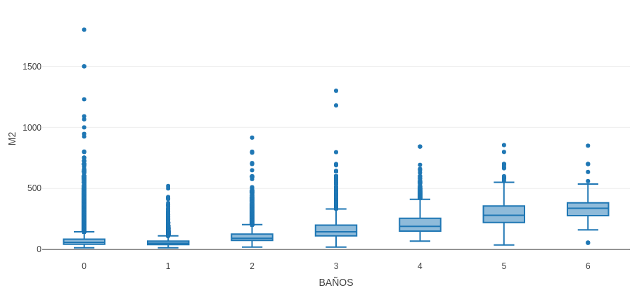
This graphic was made with an R library that allows to interact with the graphic (it is not possible to interact here because it is only an image), being very useful to observe the limit values of each box. What the graph showed is that each square meter (M2) range often has the following number of bathrooms:
Between 14 and 69: 1 bathroom.
Between 70 and 118: 2 bathrooms.
Between 119 and 175: 3 bathrooms.
Between 176 and 238: 4 bathrooms.
Between 239 and 310: 5 bathrooms.
From 311 onwards: 6 bathrooms.
It should be noted that in the data set, in addition to the 0 bathrooms, we mentioned that there were also a few erroneous data that ranged from 7 to thousands of bathrooms. This means that it was necessary to establish an upper limit to the number of acceptable baths. To do this, those departments of the city that have the largest possible number of bathrooms were investigated, to which it was observed that there are no apartments with more than 6 bathrooms. In addition, we note that this makes sense when observing the data set, since the more baths, the fewer observations are on the set, this means that starting from 1 bath, the number of observations was decreasing faster and faster until 6 baths (with 350 observations approximately), and then in the 7 baths he made a great jump (from 350 to about 5 observations), concluding that there is the maximum limit.
- Rooms: The same thing happened with the rooms as with the bathrooms, either values with NA, with 0 rooms, with thousands, etc. Applying the same method that we did with the bathrooms, we predict the number of rooms according to the square meter by means of the following boxplot:
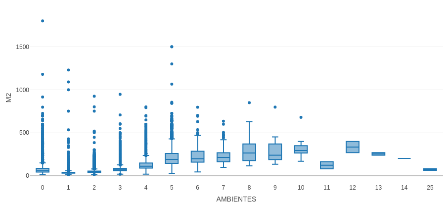
The boxplot graph shows that we could predict up to 6 rooms, since with more rooms we have few data and probably erroneous, since there are departments of many rooms with few square meters, which does not make sense. With this graph the number of rooms for the following ranges of square meters was estimated:
Between 14 and 42: 1 room.
Between 43 and 59: 2 rooms.
Between 60 and 89: 3 rooms.
Between 90 and 149: 4 rooms.
Between 150 and 260: 5 rooms.
Between 261 and 285: 6 rooms.
<br / >For the rest of the square meters, that is 285 onwards, we eliminate them since they cover a few hundred data.
- Neighborhood: No NA values were found but some typing errors that had to be corrected, such as 'NUNES' for 'NUÑEZ', 'MONSERRAT' for 'MONTSERRAT', etc.
THIRD STAGE
In the third stage of the process, the points of interest close to each department were added, be they bus stops, subways, trains, pharmacies, health centers, police stations, etc. This gives us an idea about the location of each department, that is if it is in a central or commercial area or is far from the center, which differs in the price of sales. To do this, a radius of 5 blocks around each department was established to then observe the points of interest that fall within the area, representing the places close to the department. Below is an example of this approach:
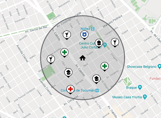
In this way, in the dataset, each department will have a column for each point of interest in which it indicates the quantity of each of these places within the radius of 5 blocks, showing which points of interest are near the department, unless of 5 blocks. This shows an idea about the location of the department, since the more points of interest are within the radius, the more central is the location area.
Once the processing of the data is finished, we group them by census radius. The main idea of grouping the database is because, since we are going to compare the price variation of the square meter year after year, we will not be able to count on the same departments in each year since there are departments that are sold while, on the other hand, new apartments for sale arise. Due to this reason, the comparison will be made between different groups.
For this we have a database of census radius from soil surveys that contains information such as latitude, longitude, location, group, population, homes, etc. that will be unified with the database of the sales of departments generated previously by the longitude and latitude whose data have both databases in common. In this way, the database of census radius will allow us to group the database in 3371 groups.
Once the databases are unified, we group the data by 'YEAR' and by 'GROUP', and for each of them we obtain the average of the square meters, dollars, price per square meter, rooms, basement, garage, bathroom, laundry, balcony, terrace and yard. As for the number of nearby places of interest, we use the sum of them for the grouping.
When obtaining these groups, for each group, we take the price variation per square meter year to year, and then calculate the average of the variations of the years 2007-2015. We use averages because there are several groups where they do not have any of the annual variations, because there are no departments in the group in any of the observed years.
With the base already grouped, we take the average of the variations of the years 2007-2015, we order them in a decreasing way and, as in the introduction we mention to defining the threshold as the 95th percentile, we take the last 5% of the whole dataset (corresponding to the higher averages of variations) and we replace them with 1, while the rest (the first 95% of the dataset) we replace them with 0. These replacements were carried out in this way because this variable will be used by the model predictive as an output value to predict the values (1 or 0), since the machine learning algorithms usually predict values of 1 or 0, or a value between both.
Then we divided the data set into two parts, one for the training set that covers the years 2007-2014, and another for the tests set that covers the year 2015. The model will use the training set to train or learn the data through the input values (rooms, bathrooms, square meters, etc.) and the output values (average of price variations), and then, through the tests set, it will predict the average of price variations of 2015 through the values of entry according to the training previously done. These predictions will be compared with the real values of the averages of variations of 2015 that we already had before building the model to give an idea about the proximity of the predicted values with the real values through statistical data.
Finally, we ran the model using random forest with XGBoost and made different samples for each modification of the model. In the best results, up to 96% accuracy was achieved.
Once the predictions on the average of variations of 2015 have been obtained, the last step is to visualize the results using a graph. For this, a geographic visualization of the Buenos Aires city was used, indicating the locations of the departments for sale that obtained the highest price increase per square meter, that is, the highest average of variation. This is because the neighborhood or area where these departments are located are in full growth and it is very likely that in the coming years they will have higher points of interest close to each department, which implies that their price increases. In this way, it would be possible to obtain a large investment by buying a department that is in a growing area, as these results suggest.
Using the geographical visualization with the ggplot library, the following result was obtained:
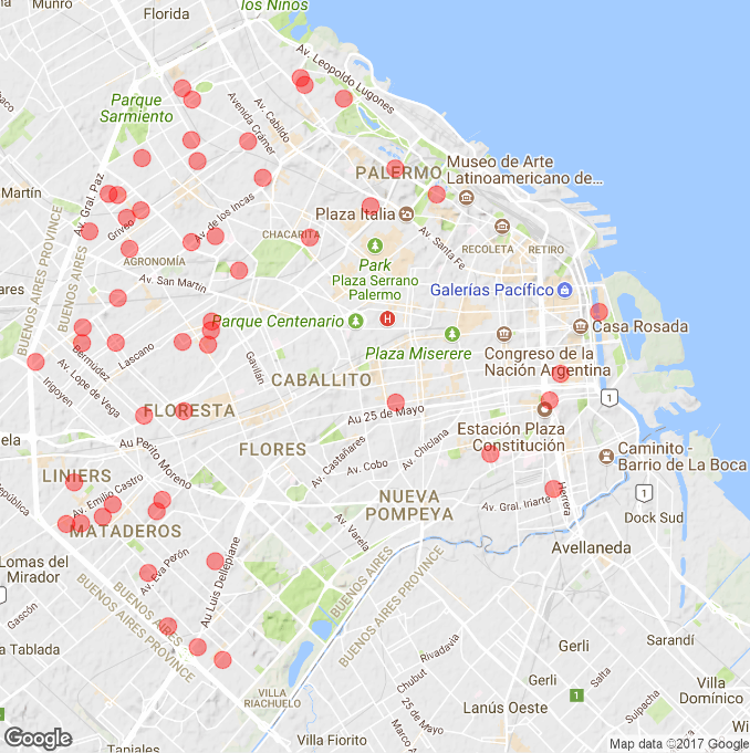
In the image you can see that the departments with the highest growth in price are mostly in the northwest and west of the city, covering neighborhoods such as Villa Pueyrredón, Liniers, Mataderos and Villa del Parque, which according to the results are the that are in full growth.